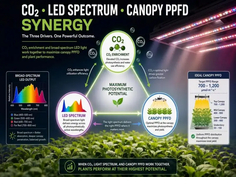
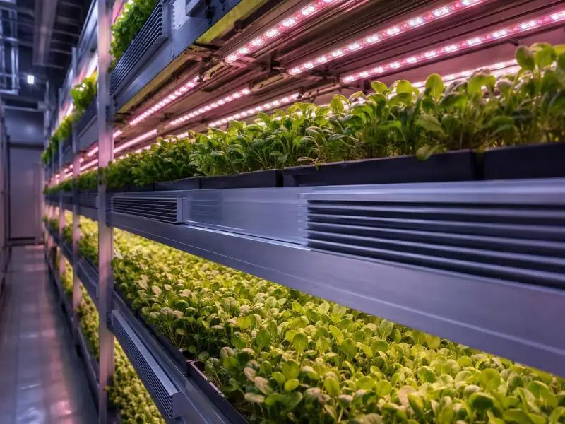
The strategy behind plant spacing vertical LEDs is a lighting-geometry decision, not a housekeeping one. The distance between bars, the gap to the canopy, and the plant’s own footprint set how evenly photons land across a tray, and that evenness feeds directly into yield per square metre and energy per kilogram. Four criteria decide a layout: the daily light integral (DLI, the total photons delivered per square metre per day) the crop needs, the photosynthetic photon flux density (PPFD, the instantaneous photon flux in µmol·m⁻²·s⁻¹) that delivers it, the uniformity you can prove by measurement, and the airflow and cooling the resulting density demands.
This guide works through each in order, then shows how to defend the layout with density trials and kWh per kilogram tracking. It was last reviewed in 2026 and reflects the standards editions currently in force.
Start from DLI and PPFD When Planning Plant Spacing Vertical LEDs
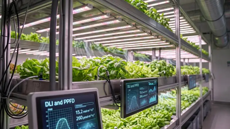
The DLI target comes first because it fixes the PPFD the array must deliver, and the PPFD fixes how much heat and electricity each tier carries. Virginia Cooperative Extension’s DLI guide gives suggested average DLI bands by crop: microgreens 9–12, lettuce 12–17, parsley 10–15, cilantro 15–20, basil 15–25, and tomato 20–30 mol·m⁻²·d⁻¹, with seedlings and cuttings at 5–10 (Virginia Cooperative Extension, 2025 revision). The same guide states plainly that the correct DLI is “somewhat subjective and not a fixed value,” and that managing DLI carries costs, so the economic side of a light level matters as much as the agronomic target.
Crop-Specific DLI Bands and Photoperiod
Treat the bands as ranges to schedule within, not setpoints to hit exactly. The guide notes that fruiting crops can need nearly double or triple the DLI of some leafy greens, which is why a tomato tier and a lettuce tier cannot share a photoperiod without different PPFD. Photoperiod is the second lever: the same DLI can be delivered by higher PPFD over fewer hours or lower PPFD over more, and the guide’s operating-hours table shows a 200 µmol·m⁻²·s⁻¹ array reaching roughly 9 mol·m⁻²·d⁻¹ at 12 hours and 12 mol·m⁻²·d⁻¹ at 16 hours. Longer photoperiods spread the electrical load but extend the hours the tier’s cooling must run.
Derive PPFD to Meet DLI with Lowest Sensible Load
The conversion is arithmetic: DLI = PPFD × 3,600 × operating hours ÷ 1,000,000, where 3,600 converts seconds to hours (Virginia Cooperative Extension, 2025 revision). The 0.0036 factor is simply 3,600 ÷ 1,000,000, so PPFD = DLI ÷ (hours × 0.0036). The guide’s worked example, 200 µmol·m⁻²·s⁻¹ over 16 hours, gives 11.5 mol·m⁻²·d⁻¹, which it describes as sufficient for seedlings through bedding plants but insufficient for most fruiting crops.
Run the derivation backwards for each tier before choosing fixtures. A lettuce target of 15 mol·m⁻²·d⁻¹ at 16 hours needs about 260 µmol·m⁻²·s⁻¹; the same target at 20 hours needs about 208. The lower-PPFD option usually wins on sensible heat per hour, but only if the crop tolerates the longer photoperiod, which is a cultivar question the extension guide leaves to the grower.
Set Uniformity Targets (Min:avg ≥0.80; ±10–15%)
No horticultural standards body publishes a pass/fail PPFD uniformity threshold. The min: mean ≥0.80 and coefficient of variation (CV, the standard deviation divided by the mean) of 10–15% figures are engineering convention, supported by published values rather than by a specification. USDA ARS uniformity optimisation work reports a planar array at 79% min: mean and an optimised layout at 95%, with every sample point inside ±7% of the mean (USDA ARS, 2022). A five-wavelength LED panel measured at CV 9.6% across 91 points on a 5 cm grid, excluding the outer 5 cm where light changes sharply (PMC3573946, 2012).
Set the target in the design brief as a number with a method attached, and expect to defend it with the mapping described below. LEDiL’s horticultural optics guide frames the same problem as three design questions: the distance required between luminaires, the distance required between luminaires and plants, and whether the photons are going where they are consumed (LEDiL, 2024).
Spacing Geometry under Vertical LEDs
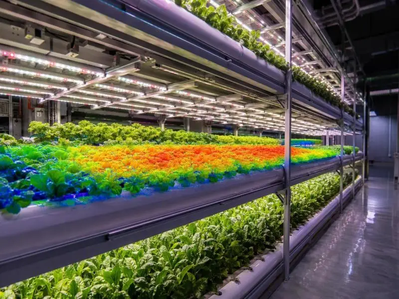
Plant spacing under vertical LEDs works as a single geometry problem: bar pitch, LED-to-canopy distance, and tray width have to be solved together, because changing any one moves the PPFD at every point on the tray. The Resource Innovation Institute’s lighting best-practice guide reports that racked vertical growing is more feasible with fixtures mounted within 12 inches of the canopy, with fixture spacing of no more than 12 inches apart below 3 ft from the canopy and up to 24 inches apart when mounted higher (Resource Innovation Institute, 2022). It also notes that continuous linear runs improve uniformity compared with grids of HID fixtures, and that uniformity is a capital and operating trade-off rather than a fixed target.
Size by Mature Canopy Diameter and Overlap Footprints
Size the plant spacing to the mature canopy, not the transplant. A crop whose canopy doubles in diameter by harvest will shade its neighbours and change the effective emitting surface the bars see, so the layout that mapped well at week one can be uneven at week four. The Resource Innovation Institute guide notes that some manufacturers model PPFD on 6-inch grids, which is a reasonable resolution for a mature canopy of that scale but too coarse for seedlings.
Overlap is where the economics sit. Closer plant spacing raises plants per square metre but increases mutual shading and lowers the light each plant intercepts, and the guide treats that as a trade-off to be modelled rather than assumed. Run the canopy-diameter calculation for the harvest week, then check the bar pitch against that footprint.
Fixture-to-Canopy Distance (15–40 cm) and Bar Layout
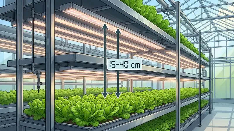
The 15–40 cm band is a design band, not a rule. The 2023 close-canopy lighting experiment tested 45, 35, 25 and 15 cm with PPFD dimmed to a constant 160 µmol·m⁻²·s⁻¹ and found fresh-biomass energy-use efficiency 2.1 times higher at 15 cm than at 45 cm (p < 0.0001), with no significant biomass difference across distances (fresh p = 0.312) (Frontiers in Plant Science, 27 July 2023). Cycle energy fell from 40 kWh at 45 cm to 31, 25, and 20 kWh at 35, 25, and 15 cm. That is one small proof-of-concept study on lettuce over a 15-day cycle, and it does not establish 15 cm as an optimum for other crops or fixtures.
The physics caveat matters more than the number. DOE/USDA-ARS on near-field modelling states that for fixtures less than 1 m from the target, as in vertical farms, near-field measurement and modelling are required, and that far-field modelling “will result in erroneous modeling of the intensity distribution” (U.S. DOE SSL Program and USDA-ARS, June 2022). The close-canopy paper adds that ordinary point-source inverse-square behaviour is unreliable at these distances because real arrays have extended emitting surfaces, multiple bars, overlap and reflections.
Bar layout follows from that. Continuous linear runs give a more even strip than discrete points, and where a residual dark lane persists between bars, staggering alternate bar positions along the tray breaks the lane without changing the pitch. No primary source prescribes a bar-to-bar distance in centimetres for multi-tier racks, so solve the pitch from the fixture’s photometric file and verify it by mapping.
Edge Zones, Aisles, and Access Constraints
Edge zones are where uniformity fails first. LEDiL’s simulation of its DAHLIA linear platform reports 95.3% PPFD uniformity on the centre 6.2 m tray (min 36, max 39, average 38 µmol·m⁻²·s⁻¹) but 67.2% on the first and last trays (min 22, max 38, average 32) (LEDiL, 2024). The end trays lose roughly a third of their uniformity to the boundary, and no amount of centre-tray tuning recovers it.
Aisles and access set the outer boundary. A tray that must be reachable from one end has a different edge profile from one serviced from both, and the access gap is also the return path for air, which the next section picks up. Map the edge trays separately and decide whether to accept the lower uniformity, add a bar, or shorten the growing run.
Validate Uniform PPFD and DLI
Validation is a measurement procedure with a written output, not a simulation screenshot. A defensible report states three ratios together, because each hides a different error: min:max, min:mean and 1 − σ/mean, where σ is the standard deviation (Harbick & Mattson, Acta Hortic. 1337, 2022). The same work used the maximum of min/mean and mean/max as its optimisation criterion and compared every point against a ±7% band around the mean.
PPFD Mapping Grids, Sensor Placement, and Metrics
PPFD uniformity mapping starts with grid resolution. The 91-point panel used a 5 cm grid across x = ±30 cm and y = ±15 cm at 17.3 cm below the emitting surface, and excluded the outer 5 cm because light changed sharply there (PMC3573946, 2012). A coarser grid will average away exactly the edge behaviour you are trying to catch.
Sensor choice is part of the method. LI-COR’s cross-sensor comparison shows a 660 nm red LED read at +1.9% by the LI-190R and +2.7% by the SQ-500, while an older SQ-110 underestimates the same LED by 36.3% (LI-COR Biosciences, current page). Apogee’s LED spectral-error table puts its own sensors within 8% overall but at −10.7% in the blue band and +5.8% in the green (Apogee Instruments, current page). These are systematic, spectrum-specific biases, not random noise, so record the sensor model and its calibration constant with every map.
Use IES Simulations and Tier-by-Tier Checks
Simulation earns its place only if the photometric input is right. ANSI/IES LM-79-24 is the approved method for optical and electrical measurement of solid-state lighting products, and its reported optical quantities include photon flux, photon flux distribution, and photon efficiency (Lisun Group summary of ANSI/IES LM-79-24, 2025). ANSI/IES TM-33 for luminaire optical data defines the XML format that carries that data into design software (ANSI/IES TM-33-18, 2018, revised 2023).
Two limits apply. First, the near-field caveat above: a far-field simulation of a 20 cm gap is the wrong model. Second, simulation is a prediction to be checked. The USDA ARS array’s quantum-sensor field measurements matched predicted PPFD within 2 µmol·m⁻²·s⁻¹, which is the standard to hold a simulation to (USDA ARS, 2022). Check every tier, not just the middle one: a 2025 measurement of light heterogeneity across 256 tray positions found PAR ranging 263–568 µmol·m⁻²·s⁻¹ at tray level, partly because two fixtures sat toward the front and one toward the back (PMC12277203, 10 July 2025).
Commissioning Steps and Dimming Strategies
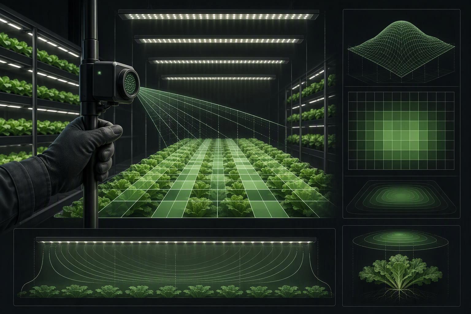
Commission in a fixed order so the record is reproducible. First, confirm the fixture’s LM-79 report and TM-33 file match the installed product and driver configuration. Second, map the empty tray on the agreed grid and compute min: max, min: mean, and 1 − σ/mean per tier. Third, compare the map against the simulation and investigate any point that differs by more than the 2 µmol·m⁻²·s⁻¹ tolerance the USDA ARS field check achieved. Fourth, repeat the map with plants in place, because a canopy changes the reflecting surface.
Dimming is the correction tool once the map exists. Per-fixture dimming can flatten a residual hotspot without moving hardware, and the USDA ARS work used PPFD modulation of individual luminaires as an alternative to non-planar mounting (USDA ARS, 2022). The same capability serves energy scheduling, since LEDs can be instantly dimmed and switched in response to changing conditions (U.S. DOE SSL Program and USDA-ARS, June 2022). Confirm the racking and controller support per-fixture dimming before specifying it; no source demonstrates uniformity dimming and energy dimming running on one controller at commercial scale.
Microclimate and HVAC Constraints
Spacing that improves light uniformity can damage the microclimate, because the same gap that puts photons closer to the canopy also removes the space air used to move through. The 2023 close-canopy lighting experiment notes that reflective curtains can enclose each growth compartment and reflect escaped photons back into it, while closer separation distances of 15–25 cm were tested (Frontiers in Plant Science, 27 July 2023). Its recommendation is controlled-velocity vertical airflow around the lamps and through the tray supports.
Air Velocity Ranges (0.3–0.8 m·s⁻¹) and Supply-to-Return Paths
The verified design band is wider than the 0.3–0.8 m·s⁻¹ figure often quoted. CFD work on multi-tier airflow sets the canopy air-velocity band for multi-tier lettuce at 0.3–1.0 m·s⁻¹ and states that velocities below 0.3 or above 1.0 m·s⁻¹ should be avoided (Zhang & Kacira, Biosystems Engineering, 2016). Treat 0.3 m·s⁻¹ as the hard floor and 1.0 as the ceiling; designed systems tend to land in the middle, and the paper’s two-perforated-tube design achieved an average of 0.42 m·s⁻¹ at the canopy.
Uniformity of air matters as much as its average. The same CFD study reports canopy air-speed coefficients of variation of 44–51% across its designs, with two perforated tubes beating one (CV 44% versus 51%) (Zhang & Kacira, Biosystems Engineering, 2016). Supply-to-return paths should therefore be drawn per tier, with the return not competing with the aisle access the spacing section already constrained.
VPD by Stage and Dew Point Control in Dense Tiers
Vapor pressure deficit (VPD, the difference between saturation and actual vapour pressure) is the control variable that ties temperature and humidity together, and dense tiers make it harder to hold. A high-humidity leaf-burn study found canopy air velocity in its plant factory “almost zero,” with strong vertical gradients producing humidity and temperature non-uniformity that drove tip burn in flowering Chinese cabbage (Kang et al., PMC9651049, 2022). Raising canopy relative humidity from 70% to 90% prevented the leaf burn that light treatments did not fix, which points at the moisture balance rather than the light recipe.
No extension service or peer-reviewed primary source with stage-specific VPD bands in kPa was verified for this guide, and the kPa-by-stage tables circulating online trace to grower calculators and vendor charts. Control dew point instead: keep the dew point below the canopy temperature by a margin the cooling coil can hold, and let the airflow numbers above do the mixing. The close-canopy paper notes that controlled vertical airflow can raise VPD and help prevent lettuce tip burn (Frontiers in Plant Science, 27 July 2023).
Thermal and Latent Load Per Tier and Driver Placement
Every tier carries its own sensible and latent load, and the spacing decision changes both. Closer bars at lower power cut cycle energy, as the 40 to 20 kWh result shows, but the heat still enters the tier, and the close-canopy paper notes that LED fixtures decouple light generation from heat generation, which allows better control of heating, cooling, and humidity (U.S. DOE SSL Program and USDA-ARS, June 2022). Driver placement is part of the thermal design: a driver inside the tier adds its losses to the canopy load, while a remote driver moves that load to a space the HVAC already serves.
Size the cooling per tier from the fixture power and the latent load the crop generates, not from a whole-room average. A 2026 scenario model of vertical-farm economics treats lighting as the dominant energy consumer in every scenario and models climate control separately, which is the right structure for a per-tier load sheet (Meeuws et al., Frontiers in Sustainable Food Systems, 2026).
Trials and ROI Decisions
The layout is only defensible once a density trial shows what it earns per square metre and per kilowatt-hour. kWh per kg vertical farming is the metric that lets a spacing change be compared with a lighting or HVAC change on the same basis, and the published benchmarks are wide enough that only your own trial settles it.
Density Trials: Compare Spacing for Marketable Yield Per m²
Design the trial as a spacing comparison at constant DLI, so the only variable is geometry. Hold PPFD and photoperiod fixed across the plots, vary plant spacing and bar pitch, and record marketable yield per square metre rather than total biomass, since the USDA ARS work notes that uneven growth may affect sales or data collection (USDA ARS, 2022). Run at least one full cycle per plot and map PPFD at the start of each.
| Trial variable | Hold constant | Record per plot |
|---|---|---|
| Plant spacing (canopy diameter) | DLI, photoperiod, VPD setpoint | Marketable kg·m⁻², cull rate |
| Bar pitch and layout | Fixture model, dimming schedule | min: mean, min: max, 1 − σ/mean |
| Fixture-to-canopy distance | PPFD at canopy | kWh per cycle, kWh·kg⁻¹ |
| Airflow design | Cooling setpoint | Canopy velocity, tipburn incidence |
The 2026 scenario model gives a sense of the yield range a trial is trying to move within: modelled lettuce output runs 78–330 kg fresh weight m⁻² yr⁻¹ per net growing area, against a Dutch greenhouse benchmark of 68 (Meeuws et al., Frontiers in Sustainable Food Systems, 2026). Those are scenario outputs for a hypothetical Dutch farm, not measured commercial results, so use them to frame the trial, not to set its target.
Track kWh per kg and Utility Incentives with DLC-Qualified Fixtures
Start from the measured benchmark, not the modelled one. A 2024 benchmarking review of vertical-farm energy use reports lettuce specific energy concentrated at 10–18 kWh·kg⁻¹, with review-reported facility-size averages of 34.2 kWh·kg⁻¹ below 1,000 m², 14.9 kWh·kg⁻¹ at 1,000–5,000 m² and 8.3 kWh·kg⁻¹ above 5,000 m² (Miserocchi & Franco, Thermal Science and Engineering Progress, 2024/2025). Those size-tier averages are attributed in the review to an earlier reference, so label them as review-reported rather than as the review’s own measurements.
For comparison, the 2026 model puts lettuce at 7.83 kWh·kg⁻¹ in its current scenario and 2.31 kWh·kg⁻¹ in its next-generation scenario, against a Dutch greenhouse benchmark of 3.81 kWh·kg⁻¹ (Meeuws et al., Frontiers in Sustainable Food Systems, 2026). The measured range is the more authoritative for a real facility; the model is a target-setting tool, which its authors state explicitly.
Fixture qualification enters here. DLC Horticultural Technical Requirements V4.0 sets a minimum photosynthetic photon efficacy (PPE) of 2.5 µmol·J⁻¹ over 400–700 nm, with a −5% tolerance so test reports at or above 2.38 µmol·J⁻¹ are accepted, and a Q90 photon-flux maintenance of at least 36,000 hours by LM-80/TM-21 or LM-84/TM-28 (DesignLights Consortium, 11 March 2025). Applications opened on 18 April 2025, and V3.0 products were delisted on 5 January 2026, so a quote referencing the V3.0 listing is out of date.
Listing is not a rebate. The DLC’s V4.0 programme page describes a product-verification list, and eligibility for a utility incentive depends on the local program, customer class, and application (DesignLights Consortium, 2025). No current utility program document with actual $/watt or $/fixture rates was verified for this guide, so check the local program directly rather than assuming a listed fixture qualifies.
Standardize Settings Across Sites for Predictable Outcomes
Multi-site consistency depends on writing the settings down as a specification, not as a habit. The DOE/USDA-ARS meeting summary notes that standardized horticultural performance labeling has been advocated but “has not yet been generally adopted by or required of” the industry, which is why Qualified Products List listing is the de facto verification gate (U.S. DOE SSL Program and USDA-ARS, June 2022). A site specification that names the fixture, the LM-79 report, the mapping grid, the uniformity metrics, and the airflow band gives every site the same reference.
The energy context justifies the discipline: US horticultural lighting consumes an estimated 9.6 TWh of site electricity per year, and converting all of it to LED could save about one-third, roughly $350 million (U.S. DOE SSL Program and USDA-ARS, June 2022). A layout standard that holds kWh·kg⁻¹ across sites is how that saving survives commissioning.
Conclusion
Plant spacing under vertical LEDs resolves into four linked decisions: the DLI the crop needs, the PPFD and photoperiod that deliver it at the lowest sensible load, the uniformity you can prove with min: max, min: mean and 1 − σ/mean on a documented grid, and the airflow and cooling the resulting density requires. The evidence is strongest on the arithmetic and the metrics, and thinnest on any single recommended distance: the 2.1-fold energy result at 15 cm comes from one small lettuce study, and no primary source prescribes a bar pitch in centimetres for multi-tier racks.
The practical next step is a layout review before the next rack goes up. Take the crop’s DLI band, derive the PPFD at your intended photoperiod, map one tier on a 5 cm grid, and compare the result against the ±7% band the USDA ARS work used. If the map and the simulation disagree, the simulation is wrong until proven otherwise.
About the publisher. SLTMAKS makes full-spectrum LED grow lights for growers from hobbyists to commercial operators, so it sells lighting that this guide’s spacing and PPFD decisions bear on. It has a commercial interest in how lighting layouts are chosen, and readers should weigh its perspective with that in mind. The guidance above does not depend on its products.
FAQ
What is the ideal distance between vertical LED bars and the plant canopy?
Most multi-tier racks end up with 15–40 cm (6–16 in) from the emitting surface to the mature canopy, and the Resource Innovation Institute’s lighting guide puts fixtures within 12 in (about 30 cm) of the canopy for racked vertical growing. Treat that as a starting point, not a rule: the 2023 close-canopy trial found 15 cm cut cycle energy from 40 kWh at 45 cm to 20 kWh at the same 160 µmol·m⁻²·s⁻¹, with no significant biomass loss on lettuce. Set the final height by measuring PPFD at canopy level, then confirm the crop tolerates the resulting heat and airflow at that gap.
What PPFD uniformity should I target on a vertical tier?
Aim for min:mean ≥0.80, with a coefficient of variation of 10–15% or lower. A USDA ARS planar array sat at 79% before optimisation and 95% afterwards, so 0.80 is a floor rather than a stretch. Measure on a 5 cm grid at canopy height and lean toward 0.85 where crop consistency drives price. Edge trays will always test lower — LEDiL’s DAHLIA simulation dropped from 95.3% on the centre tray to 67.2% on the first and last — so decide in advance whether to accept that, add a bar, or shorten the growing run.
How do I convert my PPFD target into a DLI figure?
Use DLI = PPFD × photoperiod hours × 0.0036, where the 0.0036 factor converts µmol·m⁻²·s⁻¹ and hours into mol·m⁻²·d⁻¹. A canopy at 250 µmol·m⁻²·s⁻¹ for 16 hours delivers 14.4 mol·m⁻²·d⁻¹, which sits inside the 12–17 band Virginia Cooperative Extension suggests for lettuce. Run it backwards to pick a fixture: a 15 mol·m⁻²·d⁻¹ target needs about 260 µmol·m⁻²·s⁻¹ at 16 hours but only about 208 at 20 hours. The extended photoperiod saves PPFD, not cooling hours.