Supplemental Lighting for Strawberry Winter Production in Northern Climates

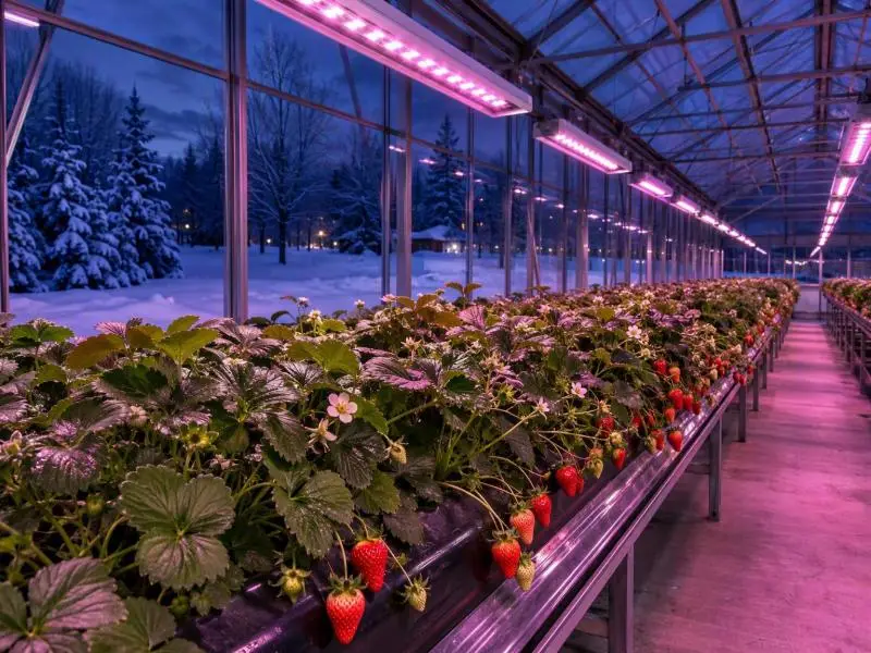
A northern winter greenhouse does not fail strawberry production because it is cold. It fails because the photons run out. Under overcast winter conditions, outdoor daily light integral (DLI) can fall below 5 mol/m²/d, and the greenhouse structure and glazing remove another 30–50% of what arrives (Ohio State, photosynthetic lighting). Against an in-house minimum of 10–12 mol/m²/d and an optimum of 20–25 mol/m²/d, that leaves a structural deficit no heating setpoint can close.

This guide works from published extension and research material rather than first-hand trial data. It follows the sequence a grower actually works through: define the deficit, set a DLI target, measure what the house already delivers, choose a photoperiod strategy, size fixtures, cost the delivered mole, fix distribution and sensor placement, integrate with climate control, design against the known failure modes, and commission the system against measured results. Every number below is either attributed to a source or flagged as an assumption to replace with your own site data.

What Strawberry Supplemental Lighting Has to Solve in a Northern Winter

Two different jobs get bundled under “supplemental lighting,” and confusing them is the most common early design error.

The first job is photosynthetic: raise the total daily photon dose so the crop can build yield. Fruiting-crop productivity typically tracks cumulative light in a roughly linear relationship, which is why DLI is the working currency for this job (Ohio State). The second job is photoperiodic: deliver a small, precisely timed signal that changes how the plant develops — breaking semi-dormancy, sustaining flower initiation in facultative long-day types, or, if mishandled, suppressing it in short-day types. The intensity difference between the two jobs is roughly two orders of magnitude, so a system designed for one will not perform the other by accident.

The deficit itself is structural, not weather-driven. At 40°N, available radiation on 21 June is about three times that on 21 December; put another way, the light available for a November–January winter crop is only about one third of the summer figure (Roberts, Wisconsin Extension). Layer glazing reflection, structural shading, overhead equipment and thermal screens on top, and a northern house in December is operating far below the crop’s minimum even on a clear day. A run of cloudy weather makes it worse, but clearing skies do not fix it.

That framing matters for procurement. You are not buying insurance against occasional dull weeks; you are buying a predictable daily photon supplement for a four-to-six-month period, and the economics have to work across that whole period.

Setting a DLI Target: Minimum, Optimum and the Stress Ceiling

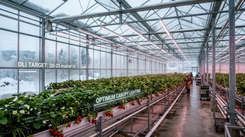
Ohio State extension guidance for greenhouse strawberry sets the minimum in-house DLI at 10–12 mol/m²/d and the optimum at 20–25 mol/m²/d, with DLI above 30 mol/m²/d apparently imparting stress to the plants (Ohio State). Two qualifications belong with those figures.

First, they are general extension guidance for strawberry, not cultivar-specific prescriptions. Critical photoperiod, dormancy sensitivity, and light response vary by cultivar, and the same page notes that you should select photoperiod based on a cultivar’s photoperiodic type and its sensitivity to dormancy-inducing short days. Treat the range as a defensible planning envelope, not a guaranteed optimum for your genetics.

Second, the target is total, not supplemental. Solar plus electric light must sum to the target. A house that already receives 8 mol/m²/d of natural light on a bright February day needs roughly 4 mol/m²/d of supplemental light to reach a 12 mol/m²/d minimum — not 12. This is why the sizing step later in this guide begins with a measured natural DLI rather than a nameplate intensity.

For commercial planning, a published control study used a 12.6 mol/m²/d target in a commercial greenhouse and reported that the HLI-based LED strategy raised DLI to approximately 10 mol/m²/d, with fruit yield per plant up 32%, soluble solids up 21% and sugar-acid ratio up 33% relative to an unlit control (Yang et al., IJABE). Read that as evidence that a target near the lower end of the extension minimum band can produce measurable commercial response under the conditions of that trial — not as proof that 12.6 is right for your site, cultivar or market.

The stress ceiling deserves equal attention in design. A system sized to hit the optimum on a bright week, with no dimming or shutoff logic, can push a clear March canopy past 30 mol/m²/d. The ceiling is a control constraint, not just a target.

Calculating Your Greenhouse’s Natural DLI and the Deficit to Close

The calculation has three inputs and one subtraction.

Illustrative winter light budget for a northern greenhouse, using the article’s flagged assumptions (outdoor December DLI 4 mol/m²/d, canopy transmission 55%) rather than a site measurement. Delivered natural DLI is 2.2 mol/m²/d, leaving a 9.8 mol/m²/d gap to the 10–12 mol/m²/d minimum band and a 17.8 mol/m²/d gap to the 20 mol/m²/d optimum. Replace both inputs with local weather records and a canopy-level transmission measurement before sizing.

Step 1 — outdoor DLI. Use a local weather station record or a published DLI map for monthly outdoor totals. Ohio State points to the Logan and Faust interactive DLI map for monthly outdoor DLI and recommends a conservative 50% transmission assumption when converting outdoor to indoor values, noting that a new, well-designed greenhouse can reach as high as 70% (Ohio State, environment).

Step 2 — transmission, measured at canopy level. Do not adopt 50% or 70% from a page. Measure it. The Rutgers glazing workshop distinguishes transmittance measured at the glazing from transmittance measured at the canopy: the first characterizes the glazing material, the second characterizes the whole system — glazing plus structure — as it delivers light to the crop (Rutgers workshop summary). The Wisconsin Extension data make the gap concrete: a research house heavily encumbered with a movable irrigation system, heating system, and thermal screen showed a relatively low transmission value, and a 7 mm wire-glass roof transmitted 13% less light than 4 mm glass in the same facility (Roberts). Your screens, trusses, gutters, and lamps are part of your transmission factor.

Step 3 — convert logged PPFD to DLI. The e-GRO method: take the hourly µmol/m²/s averages across the 24 hours, sum them, and divide by 24 (e-GRO Alert 202). Their worked example sums 24 hourly readings to 3,243 µmol/m²/s and divides by 24 to get an average of 135 µmol/m²/s. Because the sum of hourly averages divided by 24 equals the daily total in mol/m²/d when each hourly value is treated as that hour’s average intensity, the arithmetic is a direct route from a logger export to a DLI figure.

Step 4 — the deficit.

Natural DLI = outdoor DLI × canopy transmission Deficit = target DLI − natural DLI

Worked example, with every input flagged as an assumption: outdoor December DLI of 4 mol/m²/d (assumption — replace with your local record), canopy transmission of 55% (assumption — replace with your measurement), giving a natural DLI of 2.2 mol/m²/d. Against a 12 mol/m²/d minimum, the deficit is 9.8 mol/m²/d. Against a 20 mol/m²/d optimum, it is 17.8 mol/m²/d. That spread is the single largest cost decision in the project, and it should be made deliberately rather than by defaulting to the optimum.

Run the calculation monthly, not annually. The deficit in October and March is small; the deficit in December and January is the one that sizes the system.

Choosing a Photoperiod Strategy: Day Extension, Night Interruption or Cyclic Lighting

Photoperiod lighting is a signal, not a photon dose. Ohio State describes the required intensity as only a few µmol/m²/s PPFD — roughly one hundredth of typical photosynthetic lighting intensity — and recommends expressing it in PPFD rather than the older watts-per-area practice, which conflated input power with irradiance at the canopy (Ohio State, photoperiodic lighting).

The three documented methods, with their timing:

• Extension lighting: 4–6 hours of light before or after the natural day length.
• Night interruption: 3–4 hours of light around midnight to break the long dark period.
• Cyclic (intermittent) lighting: repeated cycles of 15 minutes of light and 45 minutes of dark through the night, widely used in the Netherlands and Belgium in double-cropping systems.

Intensity for these applications sits at 2–3 µmol/m²/s, with a minimum of 2 µmol/m²/s cited for dormancy control (e-GRO Alert 10(6)).

Cultivar type governs whether this helps or hurts. Most North American greenhouse cultivars are facultative long-day types that develop more flowers under longer days, and where photosynthetic lighting already runs through winter, long-day conditions are created as a side effect, and dormancy rarely becomes an issue (e-GRO). Short-day (June-bearing) types are the risk case: ‘Chandler’, ‘F-127’, ‘Radiance’ and ‘Shuksan’ all showed critical photoperiods between 13 and 14 hours, meaning exposure to 13 hours or less induces flowering in vegetative plants — and prolonged long-day or cyclic lighting may suppress flowering in short-day cultivars (Ohio State, flowering basics; photoperiodic lighting). The response is also temperature-dependent: a prolonged warm spell around 26°C delayed flower development by weeks in ‘Chandler’ in one Ohio trial.

Two practical rules follow. Add extension hours before sunrise rather than after sunset, so the far-red-rich natural light at dusk — which promotes extension growth — is preserved. And when lighting short-day cultivars, start at the lower end of the optimum temperature range (for example, 16°C average daily rather than 18°C) to reduce the chance that lighting disrupts repeat flowering; some growers run a short day-extension period and stop as soon as petiole elongation confirms the plants have come out of dormancy.

Sizing Fixtures: From Target PPFD to Fixture Count and Wattage

This is where the deficit becomes steel and watts. The arithmetic is simple; the discipline is in labelling every input.

Symbolic chain:

Supplemental DLI (mol/m²/d) = supplemental PPFD (µmol/m²/s) × lit hours × 3600 ÷ 1,000,000 Power density (W/m²) = supplemental PPFD ÷ fixture efficacy (µmol/J) Fixture count = power density × lit area ÷ fixture input wattage

Worked example. Assume a target supplemental PPFD of 150 µmol/m²/s (the 100–200 µmol/m²/s band is described as typical for strawberry), 14 light hours, fixture efficacy of 3.0 µmol/J, and a 600 W fixture (all assumptions — replace with your own).

• Supplemental DLI = 150 × 14 × 3600 ÷ 1,000,000 = 7.56 mol/m²/d.
• Power density = 150 ÷ 3.0 = 50 W/m².
• For 500 m² of lit canopy: 25,000 W, or about 42 fixtures at 600 W.

Check the DLI result against the source’s own figures: at 100–200 µmol/m²/s, continuous operation for 13 hours yields 4.68–9.36 mol/m²/d, and for 16 hours yields 5.76–11.52 mol/m²/d (Ohio State). The 7.56 figure sits inside both bands, as it should.

Now close the loop against the deficit from the previous section. If the December deficit was 9.8 mol/m²/d and this configuration delivers 7.56, the system falls short — either extend the lit hours, raise PPFD, or accept a lower winter target. If the deficit was calculated against the optimum, the same system may be substantially oversized. This is the point at which the target decision from Section 2 becomes a capital cost.

Three inputs deserve scrutiny. Lit hours are constrained by photoperiod strategy and by the dark period fruiting crops need. Fixture efficacy should come from a test report at realistic operating temperature, not a datasheet peak. And the lit area is canopy area, not floor area — in a gutter or table system those differ.

What Supplemental Light Costs per Mole Delivered

The conversion that makes this tractable: 1 µmol/J equals 3.6 mol/kWh (Mattson, Cornell NEGC).

Fixture-level efficacy converted to energy per delivered mole (1 µmol/J = 3.6 mol/kWh, so kWh/mol = 1 ÷ (3.6 × µmol/J)). HPS spans 1.16–1.70 µmol/J; 2–3 µmol/J is the typical commercial LED range; 3.69 µmol/J was the best LED fixture reported by year in Mattson’s deck and is not a typical fixture. Multiply kWh/mol by your electricity price for cost per mole.

Cost per mole delivered:

Cost ($/mol) = electricity price ($/kWh) ÷ (efficacy (µmol/J) × 3.6)

At 0.12/kWh and 3.0 µmol/J: 0.12 ÷ 10.8 =0.011 per mole. At 1.5 µmol/J (typical HPS territory): 0.12 ÷ 5.4 = $0.022 per mole. The efficiency gap is the whole story — Ohio State puts conventional HPS at roughly 1.0–1.7 µmol/J against high-efficiency LEDs above 3.0 µmol/J, a two-to-threefold difference (Ohio State).

Scale it to the season. A system delivering 7.56 mol/m²/d over 500 m² for 120 winter days delivers about 453,600 mol. At $0.011/mol, that is roughly $5,000 in electricity; at $0.022/mol, roughly $10,000. Demand charges can add materially on top, since they are set by the highest usage in a single short interval during the month — simultaneous switch-on of the whole installation is the classic way to inflate them.

Comparing two fixtures. Simple payback = upfront price difference ÷ annual electricity price difference (Mattson). If fixture A costs 400 and runs at 2.8 µmol/J while fixture B costs550 and runs at 3.2 µmol/J, the $150 premium per fixture is recovered out of the annual kWh difference — which you compute from the same operating hours and the same delivered moles, not from nameplate wattage alone.

Payback on the whole installation is a different question, and an honest answer requires a locally established yield response. The published yield gains are real but conditional: +32% fruit yield per plant in one commercial greenhouse trial at a 12.6 mol/m²/d target (Yang et al.), and increased yield and fruit number across three everbearing cultivars under nighttime LED extension in a subtropical study where fruit weight and soluble solids did not change (Nakayama, Hort. J.). Neither transfers automatically to your cultivar, climate, and price point.

On efficacy ceilings: a modelled analysis puts the upper limit of LED fixture efficacy at 3.4 µmol/J for white+red fixtures and 4.1 µmol/J for blue+red, reduced by about 10% when optical protection from water and humidity is added (Kusuma & Bugbee, Horticulture Research). Those are physics ceilings for fixture design, not a shopping specification — a greenhouse fixture with ingress protection will sit below them, and the same paper notes tradeoffs between peak efficacy and cost.

Light Distribution: Targeted Canopy Lighting and Movable Systems

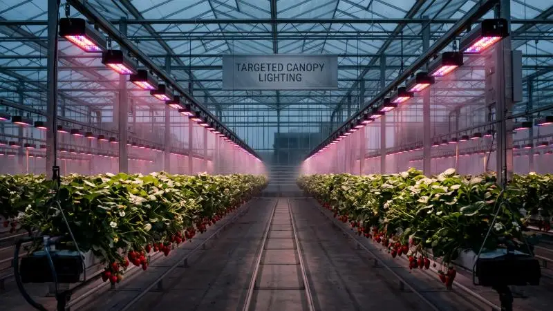
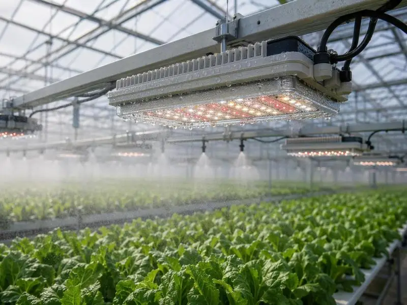
Photons that leave the fixture and land on a walkway are paid for and never absorbed. Ohio State’s illustration of a commercial strawberry operation makes the point directly: HPS distributes light over a wide horizontal plane, and in that setting much of the output is wasted illuminating the aisle (Ohio State). The recommended responses are targeted lighting over the plant canopy or a full-canopy production approach such as a movable gutter system, and Ohio State states that improving photon delivery to plants in this way can further increase light-based productivity — grams per mole — by more than 50%.

That figure is about the efficiency of converting delivered light into harvest, not about yield per fixture, and it is a strong argument for designing layout before choosing hardware.

Beam distribution and mounting height set uniformity. The Kusuma and Bugbee review notes that early LED fixtures had narrow beam angles and produced non-uniform distribution, that newer fixtures distribute photons more broadly, and that high-wattage HPS fixtures must be mounted higher above the canopy than LEDs to achieve uniform distribution (Nature).

The practical consequence: a DLI target met on average but not at the canopy is not met. A sensor in the brightest bay can report compliance while the plants under the fixture edges and between rows run below the minimum all winter. Uniformity is not an aesthetic preference; it is the difference between the design DLI and the DLI the crop actually receives.

Where to Place Quantum Sensors and How Many

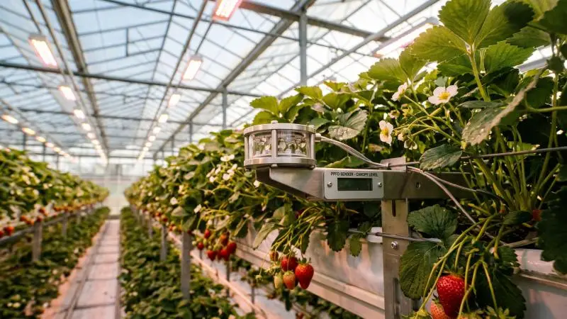
Sensor placement follows from the measurement logic already established: you are trying to represent the crop, not the building.

• Height: canopy level, per the Rutgers distinction between glazing-level and canopy-level transmittance (Rutgers). A sensor at truss height measures a light environment no leaf experiences.
• Logging interval: short and continuous. The e-GRO guidance is to record instantaneous intensity at a defined interval — once every 15 to 60 seconds is given as an example — and then calculate DLI from the logged series (e-GRO Alert 202).
• Sensor type: a multiple-diode sensor takes a reading from each diode and reports the average, giving a more representative reading than a single-diode unit. Instantaneous readings cannot substitute for integrated daily totals, because natural light changes continuously through the day.
• Position: in the crop, not the aisle — the same logic that makes walkway lighting wasteful makes walkway sensing unrepresentative.

How many? Reason from the sources of variation rather than a fixed rule. Each lighting zone, each bay with a different orientation or screen regime, and each distinct canopy type is a separate population. A single sensor in a multi-bay house with independent lighting circuits will not tell you whether the circuits are balanced. A defensible starting logic is one logged sensor per lighting zone, plus additional sensors in the zones with the highest expected variability — house edges, areas under overhead equipment, and the boundary between screened and unscreened sections. Add a handheld quantum meter for spot checks across the lit area, and use it to confirm that the fixed sensors are where the variation actually is.

Integrating Lighting with Heating, Venting and Thermal Screens

A northern winter house is a set of coupled decisions, and lighting is one of them.

Lighting adds heat, but not boiler capacity. The HLI control study measured a 1–2°C rise in strawberry canopy temperature under LED supplemental lighting (Yang et al.). That is a real effect on the crop microclimate and a real interaction with your temperature setpoints — but it is not a substitute for installed heating capacity. Cornell’s guidance is explicit that some greenhouses have historically accounted for HID waste heat and reduced boiler size accordingly, and that LEDs still provide some waste heat (Mattson). Sizing a northern house’s boiler on the assumption that lighting will carry part of the load is a design risk, not a saving.

Screens and overhead equipment cut transmission. The Wisconsin data show a heavily encumbered research house with a thermal screen, irrigation, and heating overhead delivering a relatively low transmission value (Roberts). A house that closes its screen on a cold night is also closing it on its light. The screen schedule and the lighting schedule have to be managed together.

Venting and dehumidification compete with a closed, warm house. Every air exchange in January is heat leaving the building. Lighting decisions that raise canopy temperature and transpiration change the humidity load the ventilation strategy has to handle.

Control logic. The HLI strategy in the published study is the model to copy: it calculates a target hourly light integral, compares it with the accumulated actual, and withholds supplemental light whenever measured PPFD or temperature exceeds set maxima (Yang et al.). That is a DLI-target controller, not a clock. It naturally skips lighting on a bright morning, avoids adding light and heat to an already warm canopy, and keeps the season’s total on target rather than on schedule. Where the control system supports dimming, the same logic can modulate output instead of switching fixtures in blocks.

Risks and Failure Modes to Design Against

Each of these has a documented basis or a clear operational logic, and each has a design response.

Exceeding the stress ceiling. DLI above 30 mol/m²/d appears to stress strawberry (Ohio State). A system sized for the December deficit can overshoot in March. Response: DLI-target control with a hard ceiling, and a seasonal schedule that reduces supplemental output as natural light recovers.

Uneven canopy light. Wide beam distribution and poor layout put photons on walkways and leave canopy edges below target (Ohio State; Nature). Response: targeted canopy layout, mounting height set from a uniformity measurement, and verification with a grid of spot readings before the season starts.

Snow and ice shading. Accumulation on the glazing is a transmission loss on top of an already marginal winter light budget. Response: a snow-removal procedure written into the operating plan, and DLI monitoring that detects the loss rather than assuming the schedule is being met.

Demand spikes and tariff exposure. Simultaneous switch-on sets the monthly demand charge from the highest short-interval usage (Mattson). Response: staged or staggered startup across zones, and a conversation with the utility before commissioning.

Photoperiod mistakes in short-day cultivars. Prolonged long-day or cyclic lighting may suppress flowering in short-day types, and critical photoperiods of 13–14 hours have been reported for several commercial cultivars (Ohio State; flowering basics). Response: confirm the photoperiodic type of every cultivar in the house before programming the schedule, and keep short-day blocks on a separate circuit from long-day blocks.

Target DLI versus intercepted DLI. A target met on the sensor but not at the leaf is the failure mode that hides inside a compliant report. Response: canopy-level sensing, replicated across zones, plus periodic destructive or non-destructive checks of canopy architecture — a dense, tall canopy intercepts differently from a flat one.

A Commissioning and Monitoring Routine for the First Season

The first season is a measurement exercise as much as a production season. Run these checks in order.

1. Verify installed PPFD before planting. With the natural light excluded (night, or blackout), take a grid of quantum-meter readings at canopy height across the full lit area. Compare the grid to the design PPFD and record the spread, not just the average.
2. Confirm the transmission factor. Log outdoor and indoor PPFD on the same days and compute the ratio. If your measured canopy transmission differs from the design assumption, re-run the deficit calculation before the season is committed.
3. Log DLI continuously, per zone. Use the logged-series method, not spot readings (e-GRO).
4. Compare delivered supplemental DLI against design, weekly. The gap between design and delivery is where commissioning problems show up — a mis-set controller, a shadowed zone, a screen left closed.
5. Track electricity against the cost model. Reconcile actual kWh and demand charges with the per-mole calculation from Section 6. If the model and the bill disagree, the model’s inputs were wrong.
6. Record crop response by zone. Yield, fruit number, fruit weight, soluble solids, and harvest timing, referenced to the zones with different delivered DLI. This is the only way to establish the local yield response that payback depends on.
7. Set next season’s target on evidence. The second season’s DLI target should be a decision made from the first season’s delivered-light and crop-response records, not a repeat of the initial assumption.

FAQ